The Problem

While there are police officers who risk their lives to save others, there are those who act rashly in times of panic. How do we select the right people for this stressful but critical job?

As police cadets undergo various assessments, we might have a database of their personal attributes, including physical fitness, IQ, personality traits, etc. However, we need to know:

1. Can any of these attributes be used to predict future commander potential?
2. If so, how would they rank in their prediction accuracy?
3. How do we combine multiple attributes to further improve predictions?

Besides police commander selection, prediction techniques can also be used to identify personnel on the opposite end of the spectrum – those who are likely to maladjust. Beyond HR, the applications for prediction techniques are endless: weather forecasting, stock market pricing, population dynamics, actuarial science, etc.

An Illustration

Back to our example on police commander selection. Let’s say we collect data on a group of police cadets. We have their physical fitness and IQ scores (attributes), as well as supervisor ratings on their future commander potential. While we can collect data on fitness and IQ scores at the time of recruitment, data on commander potential is based on cadets’ performance throughout training school, and is only finalized upon graduation.

It would be much better if we can predict commander potential earlier on, so that we can shortlist only the most promising candidates.

To see if any attribute can be used to predict commander potential, scatterplots come in handy:

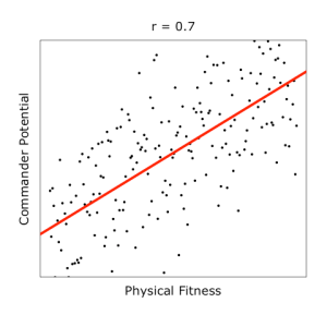
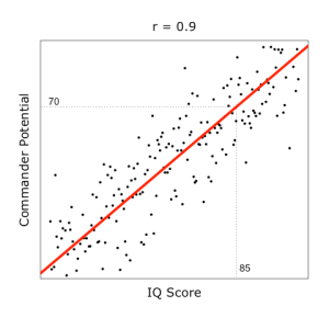
From the above plots (based on mock data for illustration purposes), we can observe trends: fitter and smarter cadets are likely to be better commanders.

Deriving these trend lines is the key to making predictions. For example, if a cadet scored 85 for IQ, the trend line predicts that he would score 70 for commander potential.

The question is, how are trend lines derived?

Technical Explanation

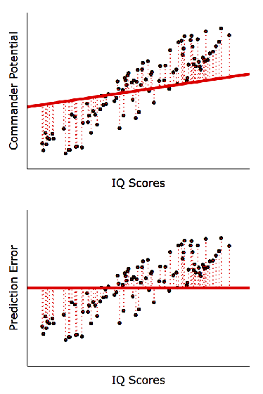
The goal of regression analysis is to derive a trend line to best fit the data (hence a regression trend line is also known as a best-fit line). This line is positioned to reduce prediction error as much as possible. The simulation below illustrates how a ill-positioned trend line would result in large prediction errors, but as the line is nudged closer to data points, prediction accuracy improves:

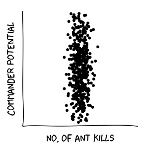
Hence, as long as we can derive a trend line between 2 variables, either variable could be predicted using the other. For contrary examples, see the plots below where predictions are not possible:

Comparing predictors:

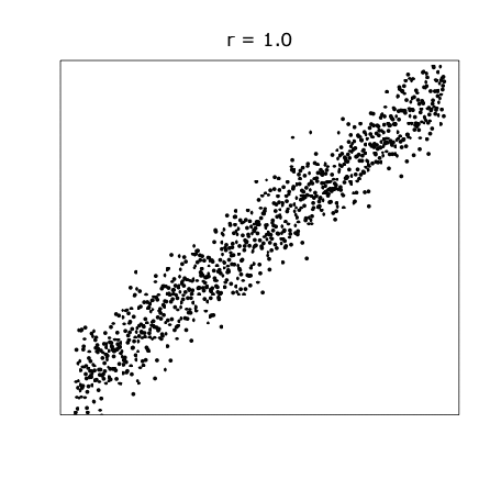
To deduce whether an attribute is a strong predictor of commander potential, we can examine how closely its data points follow the trend line. This is as measured by a correlation coefficient, r.

When data points are concentrated tightly along a trend line, it is a sign that the predictor is strong, and it will be represented by a correlation coefficient of large magnitude. For example, the correlation coefficients for fitness and IQ against commander potential were found to be r = 0.7 and r = 0.9 respectively, implying that fitness is weaker than IQ as a predictor. Intuitively, the more fluctuations in data points, the more difficult it would be to draw reliable predictions from them.

Correlation coefficients range from -1 to 1. Its positive/negative sign refers to the direction of relationship between 2 variables. As IQ increases, so does commander potential. Hence, their correlation coefficient is positive. However, if we had compared number of crimes committed against commander potential, we might expect the correlation coefficient to be negative. Here is an animation to show how scatterplots look like when variables are correlated at varying values of r:

Combining predictors:

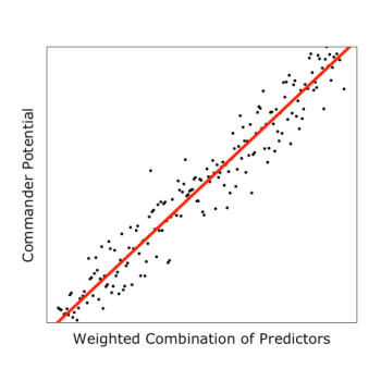
Correlation analysis tells us the strength of relationship between 2 variables, allowing us to use one variable to predict the other. However, when we want to combine multiple predictors to make predictions, we use regression analysis. Correlation analysis is equivalent to a regression analysis with one predictor.

Since we have found that both fitness and IQ scores are good predictors of commander potential, combining both attributes could improve their predictive power.

However, simply summing up both scores would not be ideal. From the results above, we know that IQ is a stronger predictor than fitness, and thus should be given more weight. But how much more?

Given that an attribute’s predictive strength is proportional to its correlation coefficient, the latter could simply be used as weights in combining attributes. So as IQ was found to be stronger than fitness as a predictor in the correlation analyses, it could be given a correspondingly heavier weight in the regression analysis.

After fitness and IQ scores are combined, we see from the plot below that the trend line becomes more apparent than if individual attributes were used alone:

Thus far, we have examined 2 distinct predictors: IQ and fitness. What if we had included a 3rd predictor, high school grades?

Even though it may be a strong predictor of commander potential on its own, the resulting weight given to high school grades in the regression analysis may be negligible. This is because high school grades overlaps with IQ scores in measuring cognitive ability, thus adding little value to overall predictive power.

Hence, it is important to select only as many distinct predictors as you need, to construct interpretable and yet simple models.

Limitation

Although regression analysis is a useful technique for making predictions, it has several drawbacks. Besides highlighting them, we examine countermeasures:

• Sensitivity to outliers. As regression analysis derives a trend line by accounting for all data points equally, a single data point with extreme values could skew the trend line significantly. Hence, before running the analysis, outliers should be identified using scatterplots.

• Distorted weights of correlated predictors. As alluded to above, the inclusion of highly-correlated predictors in a regression analysis would distort the interpretation of their weights. This problem is called multicollinearity. To ensure that predictions remain generalizable to new cases, regression models should be kept simple with as few uncorrelated predictors as needed. Alternatively, more advanced techniques such as lasso or ridge regression could be used to overcome multicollinearity.

• Straight trend lines. The type of regression analysis explained in this post is called simple linear regression. The term ‘linear’ means that the derived trend follows a straight line. However, some trends may be curved. For instance, having an average Body Mass Index (BMI) is a mark of a fit commander. Having BMI values that are too low or high could lead to undesirable health consequences. To test non-linear trends, predictors could be multiplied or exponentiated, instead of simply being added together. Alternatively, more complex techniques could be used, such as Gaussian processes.

Finally, you might have heard of the phrase “correlation does not imply causation“. To illustrate this, suppose that the amount of white hair was found to be positively correlated with commander rank. This does not mean that bleaching your hair would get you a promotion. Nor does it mean that your hair will turn white after you get promoted (although some may dispute this). Rather, commanders of higher ranks tend to be older, and you get more white hair as you age. Being mindful of how results may be misinterpreted helps to ensure the accuracy of conclusions.

Did you learn something useful today? We would be glad to inform you when we have new tutorials, so that your learning continues!

Sign up below to get bite-sized tutorials delivered to your inbox:

 

 

Copyright © 2015-Present Algobeans.com. All rights reserved. Be a cool bean.