
Editor’s Note: Due to the potential biases in machine learning models and the data that they are trained on, the blog owners Annalyn and Kenneth do not support the use of machine learning for predictive policing. This post was intended to teach random forest concepts, not to encourage its applications in law enforcement. A new post with a different application is being developed.
Can several wrongs make a right? While it may seem counter-intuitive, this is possible, sometimes even preferable, in designing predictive models for complex problems such as crime prediction.
The Problem
In the film Minority Report, police officers were able to predict and prevent murders before they happened. While current technology is nowhere near, predictive policing has been implemented in some cities to identify locations with high crime. Location-based crime records could be coupled with other data sources, such as income levels of residents, or even the weather, to forecast crime occurrence. In this chapter we build a simple random forest to forecast crime in San Francisco, California, USA.
Definition
Random forests combine the predictions of multiple decision trees. Recall from our previous chapter that in constructing a decision tree, the dataset is repeatedly divided into subtrees, guided by the best combination of variables. However, finding the right combination of variables can be difficult. For instance, a decision tree constructed based on a small sample might be not be generalizable to future, large samples. To overcome this, multiple decision trees could be constructed, by randomizing the combination and order of variables used. The aggregated result from these forest of trees would form an ensemble, known as a random forest.
Random forest predictions are often better than that from individual decision trees. The chart below compares the accuracy of a random forest to that of its 1000 constituent decision trees. Only 12 out of 1000 individual trees yielded an accuracy better than the random forest. In other words, there is a 99% certainty that predictions from a random forest would be better than that from an individual decision tree.
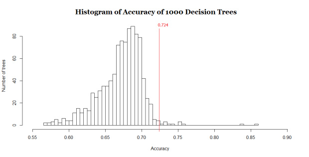
Histogram showing the accuracy of 1000 decision trees. While the average accuracy of decision trees is 67.1%, the random forest model has an accuracy of 72.4%, which is better than 99% of the decision trees.
Random forests are widely used because they are easy to implement and fast to compute. Unlike most other models, a random forest can be made more complex (by increasing the number of trees) to improve prediction accuracy without the risk of overfitting.
An Illustration
Past research show that crime tends to occur on hotter days. Open data from the San Francisco Police Department (SFPD) and National Oceanic and Atmospheric Administration (NOAA) were used to test this hypothesis. The SFPD data contains information on crimes, including location, date, and crime category. The NOAA data provides information on daily temperature and precipitation in the city.
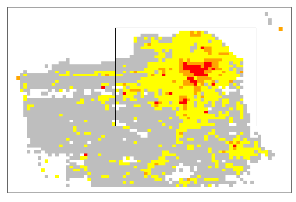
A heat map of crime levels in San Francisco. Colors indicate crime severity, which can be very low (gray), low (yellow), moderate (orange), or high (red)
From the heat map, we can see that crime occurs mainly in the boxed area north-west of the city, so we further examine this area by dividing it into smaller rectangles measuring 900ft by 700ft (260m by 220m).
Realistically, SFPD can only afford to concentrate extra patrols in certain areas due to limited manpower. Hence, the model is tasked to select about 30% of the rectangles each day that it predicts to have the highest probability of a violent crime occurring, so that SFPD can increase patrol in these areas. Data from 2014 to 2015 was used to train the model, while data in 2016 (Jan – Aug) was used to test the model’s accuracy.
A random forest of 1000 decision trees successfully predicted 72.4% of all the violent crimes that happened in 2016 (Jan – Aug). A sample of the predictions can be seen below:
Crime predictions for 7 consecutive days in 2016. Circles denote locations where a violent crime is predicted to happen. Solid circles denote correct predictions. Crosses denote locations where a violent crime happened, but was not predicted by the model.
Based on predictions illustrated above, SFPD should allocate more resources to areas coded red, and fewer to areas coded gray. While it may seem obvious that we need more patrols in areas with historically high crime, the model goes further to pinpoint crime likelihood in non-red areas. For instance, on Day 4, a crime in a gray area (lower right) was correctly predicted despite no violent crimes occuring there in the prior 3 days.
Random forest also allows us to see which variables contribute most to its prediction accuracy. Based on the chart below, crime appears to be best forecasted using crime history, location, day of the year and maximum temperature of the day.
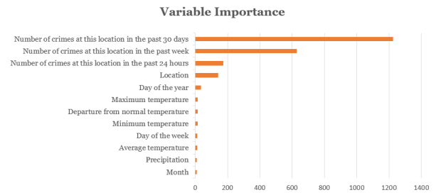
Top 12 variables contributing to the random forest’s accuracy in predicting crime.
Wisdom Of The Crowd
A random forest is an example of an ensemble, which is a combination of predictions from different models. In an ensemble, predictions could be combined either by majority-voting or by taking averages. Below is an illustration of how an ensemble formed by majority-voting yields more accurate predictions than the individual models it is based on:
Example of three individual models attempting to predict 10 outputs of either Blue or Red. The correct predictions are Blue for all 10 outputs. An ensemble formed by majority voting based on the three individual models yields the highest prediction accuracy.
As a random forest is an ensemble of multiple decision trees, it leverages “wisdom of the crowd”, and is often more accurate than any individual decision tree. This is because each individual model has its own strengths and weakness in predicting certain outputs. As there is only one correct prediction but many possible wrong predictions, individual models that yield correct predictions tend to reinforce each other, while wrong predictions cancel each other out.
For this effect to work however, models included in the ensemble must not make the same kind of mistakes. In other words, the models must be uncorrelated. This is achieved via a technique called bootstrap aggregating (bagging).
Technical Explanation
In random forest, bagging is used to create thousands of decision trees with minimal correlation. (See a recap on How Decision Trees Work.) In bagging, a random subset of the training data is selected to train each tree. Furthermore, the model randomly restricts the variables which may be used at the splits of each tree. Hence, the trees grown are dissimilar, but they still retain certain predictive power.
The diagram below shows how variables are restricted at each split:

How a tree is created in a random forest
In the above example, there are 9 variables represented by 9 colors. At each split, a subset of variables is randomly sampled from the original 9. Within this subset, the algorithm chooses the best variable for the split. The size of the subset was set to the square root of the original number of variables. Hence, in our example, this number is 3.
Limitations
Black box. Random forests are considered “black-boxes”, because they comprise randomly generated decision trees, and are not guided by explicitly guidelines in predictions. We do not know how exactly the model came to the conclusion that a violent crime would occur at a specific location, instead we only know that a majority of the 1000 decision trees thought so. This may bring about ethical concerns when used in areas like medical diagnosis.
Extrapolation. Random forests are also unable to extrapolate predictions for cases that have not been previously encountered. For example, given that a pen costs $2, 2 pens cost $4, and 3 pens cost $6, how much would 10 pens cost? A random forest would not know the answer if it had not encountered a situation with 10 pens, but a linear regression model would be able to extrapolate a trend and deduce the answer of $20.
Did you learn something useful today? We would be glad to inform you when we have new tutorials, so that your learning continues!
Sign up below to get bite-sized tutorials delivered to your inbox:

Copyright © 2015-Present Algobeans.com. All rights reserved. Be a cool bean.

Nice Explanation Thank you For giving Useful Content
Naresh I Technologies – https://nareshit.com/data-science-online-training/
LikeLike
Nice explanation Kenneth! Thanks for it.
LikeLike
Do you have example code posted anywhere?
LikeLike
It seems your assertion about extrapolation is not quite accurate. In your example of pen prices, a decision tree regressor and by extension a RF regressor would use thresholds, such as 2 pens to create edges on the graph that can be used to extrapolate unseen data. So, the 10 pen data point would simply travel down the > 2 decision path and use those weights.
In the case of linear regression, while the resulting coefficients can technically be used to extrapolate beyond the range of the training data, it’s something you really shouldn’t do, since you’d be implicitly assuming linearity beyond the range of the data. If you’ve only trained on data from 2-4 pens, you can’t assert that the # pens/price relationships stays linear after 3 pens (e.g. effect of bulk discounts etc), while a decision tree does not assume linearity.
LikeLike
WordPress mangled my reply, should read:
“…thresholds, such as less than 2 pens, 2 pens, greater than 2 pens to create edges…”
LikeLiked by 1 person
Hi Claus,
I think you made a really important point: we should not be extrapolating any machine learning models at all. I should have phrased it differently. The main takeaway is that decision trees may have some trouble generalizing to examples it has not seen before. I’ll tweak my example to elaborate this. Suppose we know that a pen costs $2, 2 pens cost $4, 3 pens cost $6, and 20 pens cost $40. A linear regression model would generate a model like (Price = 2 * Quantity) that has interpretable results, which can tell us that 10 pens cost $20. On the other hand, a decision tree might make the following classification rule: If quantity 10, then price = $40. This rule is quite optimized to the examples we were given, but it would also predict that the cost of 10 pens is $4, which is much less favourable than the regression model.
Thanks for leaving a comment! I really appreciate that and I’m happy to answer any further questions you have.
Kenneth
LikeLike
Hi Kenneth,
If that was the way decision tree regressors worked, you couldn’t even interpolate, let alone extrapolate. However, you’re correct that decision trees have problems correctly predicting out-of-sample data points.
If you plot a decision tree, in say R, you’ll see that the edges of the graph are based on greater than/less than thresholds, rather than hard equality. So, in your pen/price case, you wouldn’t have a decision path for quantity = 10, but for quantity >= 10 (e.g. if 10 was in the training set). So, by design, the tree *can* be used to extrapolate, since it readily accepts out-of-range inputs. However, the results of the prediction are not to be trusted, since the predicted values are only from the training set.
Below is a quick example in R for a decision trees to illustrate this:
library(rpart)
house = read.csv(‘http://jgscott.github.io/teaching/r/house/house.csv’)
max(house$sqft)
dt = rpart(price~sqft, house, method=’anova’)
plot(dt, uniform=TRUE,
main=”Regression Tree for Sqft “)
text(dt, use.n=TRUE, all=TRUE, cex=.7)
new = house[12,]
new
new[‘sqft’] = 4000
predict(dt, new)
As we can see, the decision tree quite happily predicts for a contrived sample house with a square foot value beyond the initial training sample.
The problems is that it assumes any house over 2,155 sqft costs $154,900 no matter what the actual square footage is.
LikeLike
Very nice and simple
But as the DT may have some options for customization such as tree nodes pruning and splits algorithms … Are there similar customizations in Random Forests ?
LikeLike
Hi Mo Elso, unfortunately the randomForest package in R does not allow such a customization. Tree pruning and splits algorithms mainly serve to tackle the problem of overfitting, but using a random forest already solves this problem. The nature of the way trees are created in a random forest would also mean that it would be computationally expensive to include these customizations, and its value would be limited. Of course, the tradeoff of using a random forest instead of a single pruned decision tree is that you get a black box model. Other customizations are available though, such as choosing the minimum size of the terminal nodes or the maximum number of terminal nodes.
LikeLiked by 1 person
Reblogged this on naveenishere.
LikeLike