
To validate the program’s effectiveness, we can design an A/B test. Such tests are used to compare results from two options, A (with training) and B (without training), thus allowing us to select the better of the two. One of the most common uses of A/B tests is to compare online adverts—whether ad A or ad B is better at attracting user clicks.

Figure 1. An A/B test weighs option A against option B.
There are five steps in an A/B test:
- Select metrics
- Identify sample
- Collect data
- Analyze data
- Make recommendations
Is our training program effective in educating people to adopt healthy living habits?
. There are multiple possible definitions for the term ‘effective‘, so we need to select the definition that aligns with goals and priorities. For example, if the goal is to secure funding to run the training, and funds are granted through an anti-obesity campaign, then measurements of body mass indices (BMI) before-and-after training could be used as a primary metric of the program’s effectiveness.

Figure 2. There are multiple ways to measure a study’s objective. For instance, body weight and temperature can both be measures of health.
Secondary metrics such as muscle mass, or test scores on food nutrition knowledge, could also be included.
Check data availability. Ensure that the necessary logistics and equipment are available for metrics to be collected, and that policies on data privacy and security can be adhered to.
Beware of contradictions between metrics. While BMI and muscle mass are both health metrics, losing weight to reach a healthy BMI could result in lower muscle mass.
Randomly sample two groups of participants. Both groups should be similar in every way possible, such as having similar distributions of gender, age and fitness levels, so that improvements observed can be more confidently attributed to training received rather than to those other factors. One group (experimental) would be trained, while the other would not (control).
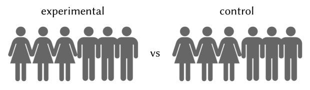
Figure 3. Experimental and control groups should preserve similar proportions for variables likely to affect results, a common one being gender.
. If the experimental group has more highly educated participants, they might be better at understanding and applying training techniques, thus artificially inflating effects of training.
Avoid ceiling effects. Participants selected for training should not already be fitness buffs, or else incremental improvements might be undetectable.
Determine sample size. Experimental and control groups should be of the same size. The total number of participants needed, also known as the sample size, depends on three factors:
- Effect size. A larger sample is needed to detect a small change. One proxy for effect size is the extent of improvement that would justify continued investment in training resources.
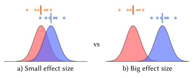
Figure 4. Comparison of distributions with different effect sizes.
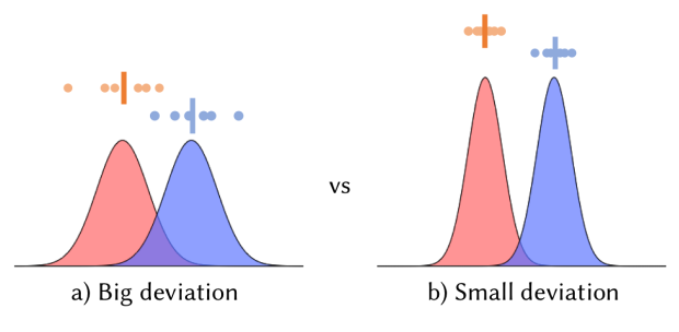
Figure 5. Comparison of distributions with different standard deviations.
- . A larger sample is needed if we want to be more certain of our results. In academia, researchers typically settle for a 95% probability that results are accurate. In practice, however, the ideal threshold depends on objectives. If false positives are costly, the confidence level could be increased.

n is the sample size needed, σ is the standard deviation, E is the effect size, and z is a value that is deduced based on the confidence level chosen. Derivation of z will be explained later.
The formula for sample size calculation makes several assumptions, such as σ being similar between experimental and control groups, and that the data spread follows a bell-curve.
Here is a demonstration of how sample size can be calculated in R. Recall that to calculate sample size, we need an estimate of deviation in the data, which can be obtained via a pilot trial. Suppose that seven people (more would be needed for accurate estimates in practice) were recruited for such a trial, and improvement in their scores on a nutrition knowledge test were recorded:
-1 0 10 20 30 40 50
sd:
# standard deviation estimate
s <- sd(c(-1,0,10,20,30,40,50))
print(s)
[1] 19.70376
If the training needs to improve scores by 5 points in order to justify funding of training resources, this can be set as the effect size desired:
# effect size desired
E <- 5
Scores could differ in two ways—either the experimental group scores higher than the control, or vice versa. To test which direction scores move would make this a two-tailed test, as shown in Figure 6. By dividing the 5% chance of error between the two tails, we get lower and upper percentile bounds of 2.5 and 97.5, which correspond to z values of -1.96 and 1.96 respectively. This means that in a symmetric bell-curve distribution centered at 0, the probability of getting a value that is within -1.96 and 1.96 is none other than 95%; only the bottom and top 2.5% would get more extreme scores. If a higher confidence level is used, the absolute value of z would increase accordingly.
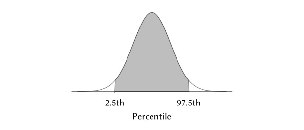
Figure 6. Probability bounds corresponding to a 95% confidence level in a two-tailed test.
z value, use the R function qnorm :
# z-statistic
z <- qnorm(.975)
print(z)
[1] 1.959964
Finally, the sample size required is calculated as follows:
# sample size required
n <- ( (z * s) / E )^2
print(n)
[1] 59.65603
Beware of Losing Control. Rather than maintaining a control group, researchers might be tempted to push all participants into the experimental training group, and then use changes in before-and-after measurements as evidence for training effectiveness. This impatience to reap rewards could backfire—without a control group, one could argue that participants’ improvements were not due to training but a result of external events.
For example, a national health campaign might have been running concurrently with the training program, from which participants picked up health tips. Without a control group, any changes in health metrics could be due to training, or external events, or both. To isolate the effect of training, a control group is necessary to parse out the impact of external events.
3. Collect Data
Determine data collection time points. To determine the effects of training, participants need to be assessed before and after training. To check how long it takes for effects to manifest and whether they last, participants need to be assessed at multiple time points after training.
Standardize data collection procedure. Ensure that participants follow the same instructions each time they are assessed, such as whether to eat or drink before their muscle mass is measured.
Prevent leaks. To avoid confounding the effects of training, remind participants in the training group not to share tips with the control group, and reassure the control group that they will receive the same training after the study if it is proven effective.
4. Analyze Data
Process missing data. Missing data can be imputed (e.g. by using averages) or labelled as a separate category. As a last resort, missing data can also be removed. However, if data is missing in a non-random manner, removing them could skew results. For instance, if participants who neglected to show up for assessments also neglected to practice what was taught in training, removing these participants could inflate observed effects of training.
Select a statistical test. Check the type of metric being analyzed to choose the right statistical test. To see changes in test scores (continuous outcome), a t-test can be used. To see whether participants are diagnosed with ailments caused by poor health choices (yes/no outcome), a χ2 -test can be used. For categorical outcomes such as ‘yes’ or ‘no’, the same formula for calculating sample size above can be used by converting counts of ‘yes’ into proportions.
Check statistical assumptions. Each statistical test makes assumptions about the data being analyzed. For example, a t-test assumes that data follows a bell-shaped distribution. Be sure to read up on the test assumptions (e.g. via Google) to ensure they are met.
Check for outliers. Data points caused by anomalies should be removed. For example, if a participant gets pregnant during the trial, her BMI would no longer be a sensible measure for her health, and her data should be excluded from analysis.
Treat unbalanced classes. For rare occurrences, such as checking whether our training program reduces the risk of heart attack among participants, additional steps would be needed. As it would be way more unlikely to experience a heart attack during the study than otherwise, observed differences would likely be minuscule and thus escape detection. Here are some possible ways to resolve this:
- Extend the study to collect more data on the rare class
- Give the rare class a heavier weight during analysis, with the risk of skewing results
- Group rare classes together, such as including other kinds of health ailments with heart attacks
- Change the evaluation metric to define health more broadly beyond heart attacks
- Under-sample the majority class of healthy individuals, selecting cases with higher risk of misclassification
- Use a statistical test suitable for rare classes, such as the Fisher’s exact test
5. Make Recommendations
Account for external events. List down events that might have influenced results. For example, a concurrent national campaign to certify restaurants based on their dishes’ nutritional values could cause a blanket improvement in diet regardless of training.
Consider scalability. Effective training might depend on small trainer-to-participant ratios. While this might be feasible for a trial, consider whether it can be replicated on a bigger scale.
Visualize findings. Use graphs and plots to communicate results, as a non-technical audience might be put off by numbers.
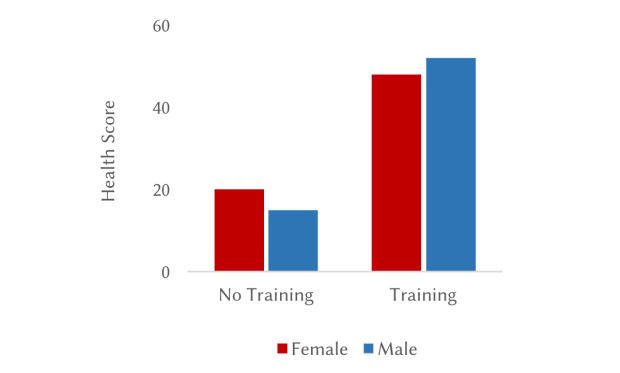
Figure 8. Example graph showing higher health scores for both female and male participants who underwent training.
Consider practical significance. We learned that a larger sample is better able to detect small differences. But this also means that tiny, inconsequential differences would be flagged as statistically significant if a study’s sample grows too large. Check, therefore, the practical significance of whether the extent of improvement justifies extra resources—is it worth conducting a training that only results in a 1% improvement in BMI?
Did you learn something useful today? We would be glad to inform you when we have new tutorials, so that your learning continues!
Sign up below to get bite-sized tutorials delivered to your inbox:

Copyright © 2015-Present Algobeans.com. All rights reserved. Be a cool bean.

Just wanted to let you know that in your R code you have “<” instead of “<"
LikeLiked by 1 person
…well, now both appear the same way so I repost with spaces in between: ” & l t ;” instead of “<"
LikeLiked by 1 person
Thanks VONJD for spotting that – fixed 🙂
LikeLike