Manchester United, under Dutch coach Louis van Gaal, has an unconventional policy on which player takes a penalty during a match. While most football teams appoint one or two players to take penalty kicks in all matches, Van Gaal has a list of five players that rotates whenever a player misses a penalty. The player that missed will go down to the bottom of the list, and will be back at the top after the four other players have missed their penalties. If we make some assumptions, we can view the problem of choosing penalty takers as a Multi-armed Bandit (MAB) problem, and we will learn whether Van Gaal’s policy is optimal.

The Setup

You have two slot machines / one-armed bandits (the number of machines can be changed). At each time you can pull the arm of either slot machines, but not both, and we assume you can play this game 2,000 times. When you play a game, you either win (get $1) or lose (get nothing). For an individual machine, the chances of winning are the same every time you play it, and it is not affected by the results of your previous plays. For machine 1, this chance is 50%, and for machine 2 it is slightly lower at 40%. The catch is, these chances are unknown to you, and so you do not know which machine will give you a higher chance of winning. What is the best way to play if you want to maximize your winnings?

This simple setup can surprisingly be applied to many different situations. For example, you may need to choose between two different kinds of ads to put on your website, but you are not sure which ad is more appealing to your customers and will thus give a better click-through rate in the long run. You may also have two experimental drugs that treat the same disease but with different chances of success.

A Simple Method

Most people would be able to think of this intuitive method to find out which machine is better. We simply play each machine 100 times, check how much we have won from each machine so far, and then decide that the machine giving you more money is the better machine. Thereafter, for the next 1,800 games, we play just that machine to maximize our winnings.

This turns out to be a pretty good strategy. On average, we are expected to win $976. As a comparison, randomly playing the machines for all 2,000 games will give $900 on average. On the other hand, if received insider information about which machine has the higher pay-out, and you play it for all 2,000 games, you will receive $1,000 on average.

To better illustrate this method, I ran four simulations of the setup, playing the game 100 times each on Machine 1 (solid line) and Machine 2 (dotted line).

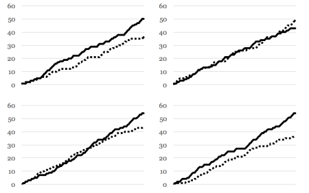
As you would expect, in most cases Machine 1 is paying out more money. In the top-right scenario however, Machine 2 actually had a higher win rate. Since the chances of winning for both machines are quite close to each other, this is not surprising. This is akin to Manchester United losing two premier league games in a row to inferior opponents – unlikely and unexpected, but it has happened before. In fact, the identification error (IE) is 8%. In 8% of the time, Machine 2 will surpass Machine 1 in pay-outs using our setup, and we will be choosing the wrong machine to play the remaining games. But since we choose the correct machine most of the time, on average we will still receive a good amount.

The Key Idea: Trade-offs

To lower the IE, we can extend the above method to play each machine 250 times at first, before deciding which is better. Surely it is much harder for Manchester United to lose three games in a row? With 250 games for each machine, the IE is now reduced to 1%. However, our average winnings decreased to $963. With a much lower IE, why didn’t our average winnings increase?

The reason is that by playing each machine 250 times instead of 100 times at the start, you are playing an additional 150 games on the weaker machine, which decreases your average winnings. Even though you are now more sure which machine is better (IE decreases from 8% to 1%), it comes at a cost.

What is the trade-off here? At the starting phase when you are playing both machines an equal number of times, you are playing sub-optimally to interact with the machines and obtain information. The IE represents a form a risk, and when you play more games at the starting phase, you are gathering more information, so your risk reduces. However, in doing so, you have less games to play optimally after the starting phase. This is often known as the trade-off between “exploration” and “exploitation”, which is a classic dilemma in reinforcement learning. Unlike the other forms of machine learning, here the learner does not know the environment and must instead interact with it to discover which actions will lead to the greatest rewards.

The best methods to solving the MAB problem strike a fine balance between exploration and exploitation. Let us consider again Van Gaal’s penalty taker approach. We can also use this strategy for our setup, which means that we stay on the winning machine and switch to the other whenever we lose. If you want to maximize your winnings, you will do well to avoid this method – it gives on average $909, which is just slightly better than playing randomly for all 2,000 games. The reason is that this method does not balance our trade-offs properly. It is perpetually exploring, i.e. it switches when faced with a poor outcome. Also, it exploits weakly as it is only concerned with how a machine performs during the previous game, rather than considering the entire past history. Nevertheless, it does still exploit somewhat, and thus it performs better than playing randomly for 2,000 games (not exploiting at all).

A Good Strategy: Epsilon-decreasing

Instead of having a single exploration phase like in the first method, we can instead spread it throughout the 2,000 games, but at a higher rate at the start and a lower rate at the end. This is what the epsilon(ε)-decreasing strategy does. At each game, we do one of the following:

• Play a machine at random (Do this with probability ε)
• Play the machine that is doing better so far (Do this with probability 1 – ε)

ε can also be viewed as the exploration probability, and it should decrease as we play more and more games. For example, we can set ε as follows:

Game number	ε
1-101	1
102	1/2
103	1/3
104	1/4
. . .	. . .
100+n	1/n

This essentially means that for we play randomly first the 101 games, and thereafter we play the better machine most of the time, and with a small random chance we play the other machine(s). The advantage of this method is that instead of sticking to one machine forever, we play the other machine(s) sometimes, just in case it turns out to be better. As time progresses, we are more sure which machine is the better one, hence we play the other machine(s) less often. So how does this method perform? On average, this method yields $984, which is an impressive result.

Using our setup, this method as an IE of 4%, but this can be lowered by controlling the values of epsilon. As such, it is essential to tune the value of epsilon to get your desired IE (see section on Limitations). What is amazing is that if we play an infinite number of games (or a very, very large number of games), this method will surely allow us to find the better machine, which does not happen for the other methods. Mathematically, we say that your expected winning rate converges to the chance that the better machine will give you a pay-out (50%).

Comparison to A/B Testing

A/B testing is a popular form of experiment that tests two different versions (A and B) of a webpage, email, or marketing material to see which version generates greater revenue. For example, a company may wish to know which of the following ads draws more customers to its website:

• Up to 50% discount on items! Shop now!
• Half-price on selected items! Find your favourite today!

A/B testing shows each ad to the same number of people, say 100, and thereafter conclude whether the click-through rate is different. When we say “different”, we are in fact using a statistical idea called “significantly different”, which means that we can be 95% sure one ad is better than the other (we can only be 100% sure if the experiment is conducted infinitely).

If A/B testing does not ring a bell, you ought to be reading this chapter again! The problem of finding which ad is better can be modelled as a MAB, and A/B testing is equivalent to the simple approach we examined earlier of playing each machine 100 times and then deciding the better machine. We also found out that the epsilon-decreasing strategy performs better than A/B testing in our setup, as it can give a higher expected winnings with a lower IE.

While the epsilon-decreasing strategy takes longer to achieve statistical significance as compared to A/B testing since it does not care much about the weaker machine after a while, that is irrelevant because the IE for this strategy is not lower. Furthermore, it is superior to A/B testing in terms of maximizing winnings. The important thing however is to take note of some limitations so that this strategy works properly for you.

Limitations

It was mentioned previously that the tuning of epsilon is essential. You need to make sure that it does not decrease too slowly (which means you will miss out on exploiting the better machine) nor decrease too quickly (which means you hastily decide which machine is better, and you will get a higher IE). Furthermore, you may not know the difference between the actual success rates of the different machines, so it may make it difficult to choose an appropriate epsilon. For example, if there is a large difference between the success rates, you will probably notice this after playing each machines a few times, so your epsilon can decrease faster. A more advanced method of deciding epsilon (Thompson sampling) will be presented in the next chapter.

The epsilon-decreasing strategy also depends on several assumptions to work well:

1. Each play of the machine will give a chance of success that is independent of all other previous plays. To illustrate how this assumption can be violated, consider an ad that is showed to the same customer multiple times in a day. For the first few times, the customer may have a low chance of clicking on it. But after seeing it repeatedly, the customer gets more curious and the chance of clicking hence increases.

2. The chance of success of playing a machine will not change over time. One ad may have a better click-through rate in the morning which decreases over the day, while another ad may have a click-through rate that increases steadily throughout the day. If this may be a problem, then it makes more sense to compare both ads after full days.

3. There is minimal delay between playing a machine and observing the result. In MAB you immediately know after playing a machine whether you won or lost. However if you are emailing your clients two different kinds of ads, they may take anywhere from one minute to three days to see the mail.

With appropriate adjustments, some of these limitations can be overcome. For some situations, it may even be irrelevant that an assumption does not hold true. Since you are ultimately comparing between two products, it may be alright if both products violate an assumption in a similar way.

Did you learn something useful today? We would be glad to inform you when we have new tutorials, so that your learning continues!

Sign up below to get bite-sized tutorials delivered to your inbox:

 

Copyright © 2015-Present Algobeans.com. All rights reserved. Be a cool bean.