
Can several wrongs make a right? While it may seem counter-intuitive, this is possible, sometimes even preferable, in designing predictive models for complex problems. Earlier in this two-part series, we looked at how kernel density plots can be used to visualize soccer shots data. We now look at how a random forest model can help us to predict the probability of a goal, with applications ranging from performance appraisal to match-fixing detection.
Association football, also known as soccer, is played by two teams of 11 players competing to shoot the ball into the opposing goal, with the objective of outscoring their opponent. Regular players may use any part of their bodies except their arms to play the ball, while goalkeepers may use their arms within the penalty area. Each game lasts 90 minutes, and each team typically makes 5 to 20 attempts to shoot the ball into the goal (“shots”), and scoring a fraction of them (“goals”).
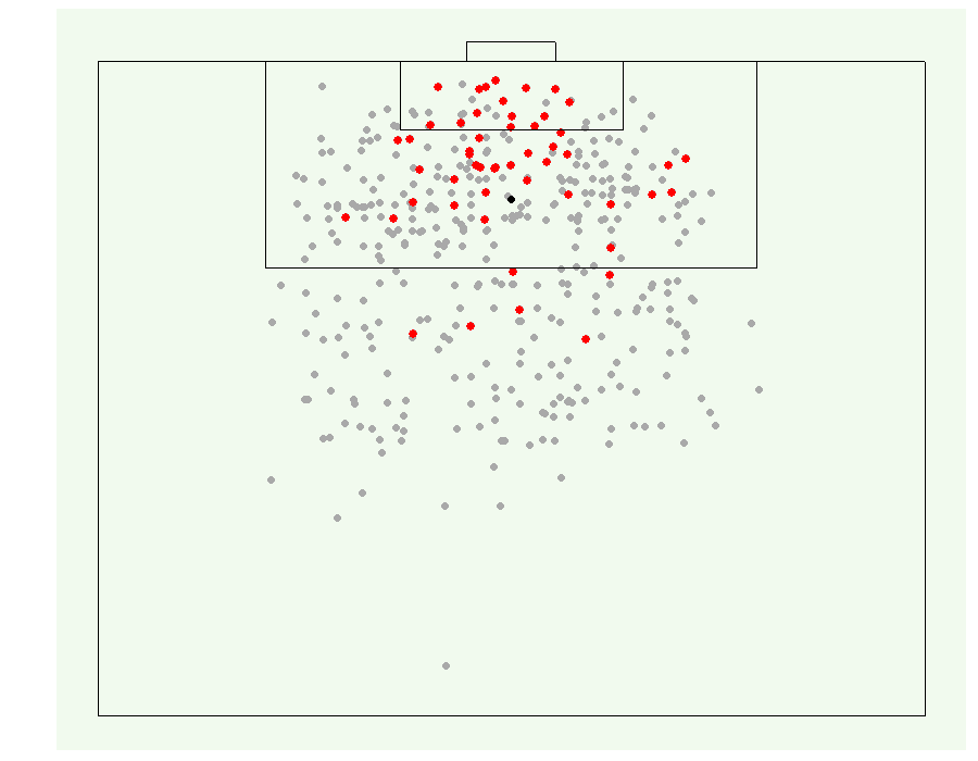
We use data on shots and goals from Wyscout, a company that compiles match videos and tags match events. The data covers all games played in the 2017-18 season across the top 5 European leagues: England, Spain, Germany, Italy, and France. Figure 1 visualizes a sample of the data—a dot represents the location where a shot was attempted, with red dots representing successful goals. The accompanying code in R is on our GitHub page.
An Illustration
Using this data, we can build a random forest model to calculate the probability of a goal. The model used predictors such as distance to the goal, visible shot angle (i.e. how much of the goal is visible), type of player who attempted the shot (i.e. defender, midfielder, or forward), match period, and strength of the shot maker’s team during offence and opponent’s team during defence (using goals/shot ratio). To predict whether a shot leads to a goal, the random forest model aggregates the results from 1000 decision trees.
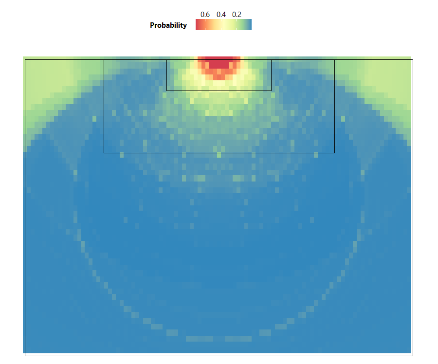
From the heatmap in Figure 2, we can see that the highest probability of scoring a goal occurs directly in front of the goal line. The high probability zone also forms a semi-circular shape, which shows an important relationship between the visible shot angle and the distance to the goal when attempting a shot—if the distance to the goal is short but the visible shot angle is small, the goalkeeper and defenders are more likely to block the shot, thus decreasing goal probability. Therefore, players on the offense should get into the high probability zone for the best chance of scoring, while defenders should prevent them from getting into this zone.
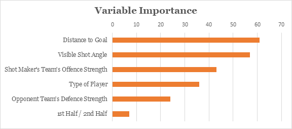
The random forest algorithm also allows us to see which variables contribute most to prediction performance. Based on Figure 3, the visible shot angle and distance to the goal have the highest influence on whether a goal is scored.
Looking at the heatmap in Figure 2, you may notice that the model reflected a 0.2 probability of scoring from the corner area of the field, which is peculiar given that it is far from the goal with limited shooting angle. This is likely due to outliers. Within this area, while most players would opt to cross the ball to a central attacker instead of shoot directly, some have unintentionally scored when making the cross.
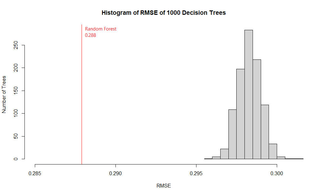
Evaluating our model using the Root Mean Square Error (RMSE) metric, which compares predicted probabilities against actual results and outputs a number from 0 (perfectly accurate) to 1 (completely inaccurate), our model’s RMSE was 0.288, implying that we can predict goal probabilities reasonably well.
Applications
Let’s re-examine the heatmap of goal probabilities in Figure 2. Notice that a player making a shot within the small box (or “6-yard box”) in front of the goal would have around 0.4 to 0.6 probability of scoring, which means 1 goal is expected for every 2 shots made within this area. If, however, the shot was made within the larger box (or “penalty box”), the player would have around 0.2 probability of scoring, which means 1 goal expected for every 5 shots made. In soccer, the concept of expected goals (or xG) has important applications:
- Performance Appraisal. If a team was expected to score 3 goals based on the circumstances of their shots, but ended up scoring only 1 actual goal, this could indicate weaknesses in their play.
- Match-fixing Detection. Multiple shots from good positions without any successful goals may indicate dishonest play, and soccer authorities use this to detect match-fixing, in conjunction with other indicators, such as players’ actions, passing intent, and suspicious betting patterns.
Commercial models that compute expected goals usually consider additional information about the circumstances of each shot, such as scenario of play (e.g. regular play, counter attacking, free kick), body part used to make the shot, and even actions that preceded the shot. This further improves the model by reducing RMSE to within 0.26 and 0.27.
Technical Explanation
A random forest is a type of ensemble, which combines predictions from many models. In an ensemble, predictions could be combined either by majority-voting or by taking averages. Figure 4 shows how an ensemble formed by majority-voting yields more accurate predictions than the individual models it is based on.
As a random forest is an ensemble of multiple decision trees, it leverages “wisdom of the crowd”, and is often more accurate than any individual decision tree. This is because each individual model has its own strengths and weakness in predicting certain outputs. As there is only one correct prediction but many possible wrong predictions, individual models that yield correct predictions tend to reinforce each other, while wrong predictions cancel each other out.
The chart in Figure 5 compares the RMSE of a random forest to that of its 1000 constituent decision trees. In our model, none of the individual trees yielded a better RMSE score than the random forest.
For ensembles to work well, models included in the ensemble must not make the same kind of mistakes. In other words, the models must be uncorrelated. This is achieved via a technique called bootstrap aggregating (bagging). In random forest bagging, a random subset of the training data is selected to train each tree. Furthermore, the model randomly restricts the variables which may be used at the splits of each tree. Hence, the trees grown are dissimilar, but they still retain certain predictive power.
Figure 6 shows how variables are restricted at each split:

In the above example, there are 9 variables represented by 9 colors. At each split, a subset of variables is randomly sampled from the original 9. Within this subset, the algorithm chooses the best variable for the split. The size of the subset was set to the square root of the original number of variables. Hence, in our example, this number is 3.
Limitations
Random forests are widely used because they are easy to implement and fast to compute. Unlike most other models, a random forest can be made more complex (by increasing the number of trees) to improve prediction performance without the risk of overfitting. However, they do have their limitations:
Black box. Random forests are considered “black-boxes”, because they comprise randomly generated decision trees, and are not guided by explicitly guidelines in predictions. We do not know how exactly the model predicted that a particular goal would happen, instead we only know that a majority of the 1000 decision trees thought so. This may bring about ethical concerns when used in areas like medical diagnosis.
Extrapolation. Random forests are also unable to extrapolate predictions for cases that have not been previously encountered. For example, given that a pen costs $2, 2 pens cost $4, and 3 pens cost $6, how much would 10 pens cost? A random forest would not know the answer if it had not encountered a situation with 10 pens, but a linear regression model would be able to extrapolate a trend and deduce the answer of $20.
Did you learn something useful today? We would be glad to inform you when we have new tutorials, so that your learning continues!
Sign up below to get bite-sized tutorials delivered to your inbox:

Data Source
Pappalardo et al., (2019) A public data set of spatio-temporal match events in soccer competitions, Nature Scientific Data 6:236, https://www.nature.com/articles/s41597-019-0247-7
We used data from the 2017/2018 season of five national first division soccer competitions in Europe: England, France, Germany, Italy, and Spain. Over 1,800 matches, 3 million events, and 4,000 players were analyzed.
Data was first collected in video format before events (e.g. shots, goals) were being tagged by operators (e.g. position of shot, player who made the shot) through a proprietary software.
